Every optimization problem (regardless of its nature) starts with an objective function subject to a set of parameters, hyperparameters, and constraints. The question is which optimization method can produce a provably optimal solution within the available time and resources.
I worked through this material before writing the paper that became arXiv:2306.10328, “Distributed Accelerated Projection-Based Consensus Decomposition” (TASK Quarterly 26(2), 2022): a QR-factorization-based variant of Accelerated Projection-Based Consensus for solving large, sparse, distributed linear systems without the full matrix inversion overhead.
Along the way I put together a short handbook combining the notation and the optimization techniques into a single pipeline. Modern tooling can pick the right strategy on its own now, but walking through the pipeline step by step still has value for understanding how the underlying model actually flows.
Mathematical Optimization Methods
The flowchart below outlines the decision process for selecting an optimization method, walked node by node in the order each check happens:
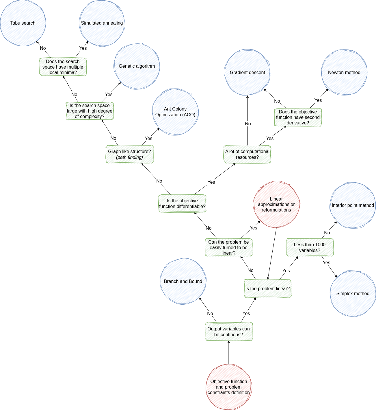
Everything starts with the variables: continuous or discrete. Discrete problems (usually integer or combinatorial) have one clear route: Branch and Bound. It divides the original problem into smaller subproblems and arranges them in a search tree, conceptually similar to tree search algorithms such as minimax with alpha–beta pruning. For each branch, it estimates the best solution that branch could possibly produce. If that estimate is no better than the best valid solution already found, the entire branch is discarded. Once every branch has been explored or ruled out, the best remaining solution is optimal.
For continuous linear problems below roughly 1000 variables, the Simplex method is the right choice. The constraints create an area of possible solutions, and the best solution is found at one of its corners. The Simplex method checks these corners one by one, moving to a nearby corner only when it improves the result. When no nearby corner gives a better result, the current solution is optimal. This resembles local search or hill climbing, but with an important distinction: ordinary hill climbing can stop at a local optimum, while linear programming has a convex feasible region and a linear objective, so a locally optimal vertex is also globally optimal.
$$ \text{minimize } c^\top x \quad \text{subject to } Ax \le b,\ x \ge 0 $$
In practice, the Simplex method is fast and reliable enough to remain widely used in applications such as logistics, scheduling, and portfolio optimization. Past roughly 1000 variables, Interior Point methods often become more efficient. Instead of moving along the edges of the feasible region, they travel through its interior. A barrier term (conceptually similar to SVM) keeps the search away from the constraint boundaries while guiding it toward the optimal solution. As the method progresses, the barrier is gradually reduced, letting the solution move closer to the boundary where the optimum may lie.
$$ \min_\theta f(\theta) - \mu \sum_i \log(-g_i(\theta)) $$
where $g_i(\theta) \le 0$ are the constraints and $\mu$ shrinks to zero as the solver converges. Iterations are more computationally expensive, but there are fewer of them than in the Simplex method.
If the problem is not linear, a log-transform, a change of variables, or a piecewise-linear approximation can sometimes reduce it back to the Simplex/Interior-Point case at little cost.
Differentiability decides the next branch. Newton’s Method uses both the gradient and second-order curvature:
$$ \theta_{k+1} = \theta_k - [\nabla^2 f(\theta_k)]^{-1} \nabla f(\theta_k) $$
It converges quadratically near a local optimum, far faster than a first-order method, but the $O(n^3)$ computation cost of inverting the Hessian matrix at every step limits it to small and medium parameter counts.
For larger problems, Gradient Descent avoids the Hessian entirely:
$$ \theta_{k+1} = \theta_k - \alpha \nabla f(\theta_k) $$
with step size $\alpha$. It uses only first-order differentiation, so each iteration is much cheaper and scales well to high-dimensional problems. This algorithm underneath is essentially in every modern training loop in deep neural networks.
Metaheuristics apply to non-differentiable objectives: they explore the solution space without relying on derivatives and can escape local optima by occasionally accepting inferior moves. For structural problems with graph structure, such as pathfinding or routing, Ant Colony Optimization is the right fit. A population of agents lays pheromone on the edges of candidate solutions. Paths that work are reinforced over time, and the colony gradually converges on good routes.
Problems without graph structure come down to scale. A large, highly complex search space calls for Genetic Algorithms. Modeled on biological evolution, they evolve a population through selection, crossover, and mutation:
$$ \text{child}_i = \begin{cases} \text{parent}_{1,i} & i < k \\ \text{parent}_{2,i} & i \ge k \end{cases} \qquad \text{gene}_i^{\prime} = \text{gene}_i + \varepsilon,\ \ \varepsilon \sim \mathcal{N}(0, \sigma^2)\ \text{ w.p. } p_m $$
Crossover swaps genetic material between two parents at a locus $k$; mutation perturbs individual genes at random with probability $p_m$. Genetic algorithms need only a fitness function (no gradients), which is what makes them so flexible.
For smaller search spaces, the decision depends on the shape of the objective landscape. A landscape with many local minima calls for Simulated Annealing, which can accept a worse move with probability $\exp(-\Delta f / T)$, where the temperature $T$ cools over the run. Early on it accepts almost anything, by the end only improvements. A landscape that is not that rough favors Tabu Search: at every step it takes the best available move even when nothing improves, while keeping a short-term memory of recent moves so it cannot simply undo itself. Unlike Simulated Annealing, Tabu Search is often implemented deterministically, though randomized variants also exist.
Viewed as a whole: continuity and linearity are decided first because they determine whether an exact or convex solver applies. Differentiability comes next because it determines whether to use gradient methods. Metaheuristics enter only once both are ruled out. Most wasted effort comes from reaching for a metaheuristic before checking whether an exact or convex method would have solved the problem faster.
Regression Analysis Algorithms
Most of the optimization problems below minimize their objective with gradient descent, a Newton-type method, or a closed-form projection. Decision trees are the main exception: rather than optimizing all parameters jointly, they build the model through a sequence of greedy splits. The sections follow the natural regression order: simple linear → multiple linear → polynomial → non-linear → logistic → multinomial logistic → classification tree → regression tree, so each one only needs to explain what differs from the last. Each section states the model function, defines the notation, gives the objective, and derives the parameter-estimation formulas.
| Property | Recommended algorithm(s) |
|---|---|
| Continuous target, linear relationship, single predictor | Simple Linear Regression |
| Continuous target, linear relationship, multiple predictors | Multiple Linear Regression |
| Continuous target, polynomial relationship | Polynomial Regression |
| Continuous target, general nonlinear relationship | Non-linear Regression |
| Continuous target, robustness/interpretability prioritized over efficiency | Regression Tree |
| Categorical target, 2 classes, smooth probability estimate required | Logistic Regression |
| Categorical target, more than 2 classes, smooth probability estimate required | Multinomial Logistic Regression |
| Categorical target, robustness/interpretability prioritized over efficiency | Classification Tree |
Simple Linear Regression
Simple linear regression fits one predictor to one response.
Model function:
$$ y = ax + b $$
| Symbol | Shape | Role |
|---|---|---|
| $y = [y_1, \ldots, y_n]^\top$ | $n \times 1$ | Labels |
| $a$ | scalar | Slope |
| $x = [x_1, \ldots, x_n]^\top$ | $n \times 1$ | Features |
| $b$ | scalar | Intercept |
Objective:
$$ \arg\min_{\hat{a}, \hat{b}} L(\hat{a}, \hat{b}) \quad \text{where} \quad L(\hat{a}, \hat{b}) = \frac{1}{n}\sum_{i=1}^n (\hat{a} x_i + \hat{b} - y_i)^2 $$
Intercept estimation using averages:
$$ \hat{b} = \bar{y} - \hat{a},\bar{x} $$
Slope estimation using projection:
$$ \frac{dL(a,b)}{da} = \frac{d\lVert(ax+b)-y\rVert^2}{da} = 2x^\top[(ax+b)-y] = 0 $$
$$ \hat{a} = \frac{\sum_i (x_i - \bar{x})(y_i - \bar{y})}{\sum_i (x_i - \bar{x})^2} $$
Multiple Linear Regression
Multiple linear regression stacks the predictors into a matrix.
Model function:
$$ y = Xw $$
| Symbol | Shape | Role |
|---|---|---|
| $y$ | $n \times 1$ | Labels |
| $X$ | $n \times (m+1)$ | Features matrix (column of $1$s prepended for the intercept) |
| $w$ | $(m+1) \times 1$ | Coefficients ($w_1$ = intercept, $w_2, \ldots, w_{m+1}$ = slopes) |
Objective:
$$ \arg\min_{\hat{w}} L(\hat{w}) \quad \text{where} \quad L(\hat{w}) = \frac{1}{n}\lVert X\hat{w} - y \rVert^2 $$
Coefficient estimation using projection (normal equation): this is the closed form the consensus paper mentioned above works around, since $(X^\top X)^{-1}$ is exactly what becomes too expensive to compute once $X$ is large, sparse, and distributed:
$$ \frac{dL(w)}{dw} = \frac{d\lVert Xw - y \rVert^2}{dw} = 2X^\top(Xw - y) = 0 $$
$$ X^\top X \hat{w} = X^\top y $$
$$ \hat{w} = (X^\top X)^{-1} X^\top y $$
Coefficient estimation using gradient descent:
$$ \nabla L(w) = \frac{2}{n} X^\top(Xw - y) $$
$$ \hat{w} \leftarrow w - \alpha \nabla L(w) \qquad \text{Repeat until convergence} $$
where $\alpha$ is the learning rate (a hyperparameter).
Polynomial Regression
Polynomial regression is multiple linear regression on polynomial features.
Model function:
$$ y = \Phi(x) w $$
where $\Phi(x)$ is the Vandermonde matrix, each row mapping a feature value $x_i$ to its polynomial expansion:
$$ \Phi(x) = \begin{bmatrix} 1 & x_1 & x_1^2 & \cdots & x_1^d \\ 1 & x_2 & x_2^2 & \cdots & x_2^d \\ \vdots & \vdots & \vdots & \ddots & \vdots \\ 1 & x_n & x_n^2 & \cdots & x_n^d \end{bmatrix} $$
| Symbol | Shape | Role |
|---|---|---|
| $y$ | $n \times 1$ | Labels |
| $\Phi(x)$ | $n \times (d+1)$ | Vandermonde feature matrix (degree $d$) |
| $w$ | $(d+1) \times 1$ | Coefficients |
Objective: The same MSE as multiple linear regression:
$$ \arg\min_{\hat{w}} L(\hat{w}) = \frac{1}{n}\sum_{i=1}^n (\Phi(x_i) \hat{w} - y_i)^2 $$
Coefficient estimation: Identical to multiple linear regression, since the Vandermonde matrix is just a specific feature matrix:
$$ \hat{w} = (\Phi^\top \Phi)^{-1} \Phi^\top y \qquad \text{(projection)} $$
$$ \hat{w} \leftarrow w - \alpha \cdot \frac{2}{n}\Phi^\top(\Phi w - y) \qquad \text{(gradient descent)} $$
Non-linear Regression
Non-linear regression covers models that are nonlinear in the parameters themselves, for example $y=ax^b$.
Model function: Linearize via a first-order Taylor approximation around the current estimate $w$:
$$ y \approx f(x, w) + J \Delta w $$
Jacobian: the $n \times m$ matrix of first partial derivatives:
$$ J_{ij} = \frac{\partial f(x_i, w)}{\partial w_j} $$
Objective:
$$ \arg\min_{\hat{w}} L(\hat{w}) \quad \text{where} \quad L(\hat{w}) = \frac{1}{n}\sum_{i=1}^n (f(x_i, \hat{w}) - y_i)^2 $$
Coefficient estimation using Gauss-Newton projection: define the residual $r = y - f(x, w)$:
$$ \frac{dL(w)}{dw} = 2J^\top(J\Delta w - r) = 0 $$
$$ \Delta w = (J^\top J)^{-1} J^\top r $$
$$ \hat{w} \leftarrow w + \Delta w \qquad \text{Repeat until } \lVert \Delta w \rVert \text{ is small} $$
Coefficient estimation using QR decomposition (applicable when $n \geq m$): decompose the Jacobian $J = Q\begin{bmatrix} R \\ 0 \end{bmatrix}$, where $Q$ is orthogonal and $R$ is upper triangular. Then $\Delta w = R^{-1}(Q_1^\top r)$, solved via back-substitution and repeated until $\lVert \Delta w \rVert$ is small.
Coefficient estimation using SVD (applicable when $n \geq m$): decompose the Jacobian $J = U \Sigma V^\top$, where $U$ is $n \times n$ orthogonal, $\Sigma$ is $n \times m$ diagonal, and $V$ is $m \times m$ orthogonal. Then $\Delta w = V \Sigma^{-1}(U^\top r)$, where $\Sigma^{-1}$ is the pseudoinverse, repeated until $\lVert \Delta w \rVert$ is small.
Logistic Regression
Logistic regression handles binary classification.
Model function: The sigmoid function applied to a linear combination:
$$ y = \sigma(Xw) = \frac{1}{1 + e^{-Xw}} $$
| Symbol | Shape | Role |
|---|---|---|
| $y$ | $n \times 1$ | Labels ($0$ or $1$) |
| $X$ | $n \times (m+1)$ | Feature matrix (with intercept column) |
| $w$ | $(m+1) \times 1$ | Coefficients |
Objective: Binary cross-entropy loss:
$$ \arg\min_{\hat{w}} L(\hat{w}) \quad \text{where} \quad L(\hat{w}) = -\frac{1}{n} \sum_{i=1}^n \left[ y_i \log \sigma(x_i \hat{w}) + (1 - y_i) \log(1 - \sigma(x_i \hat{w})) \right] $$
Coefficient estimation using Newton-Raphson: uses the Hessian $H$ and the score vector $s$:
$$ s(w) = \frac{\partial \log L(w)}{\partial w} = X^\top(y - \sigma(Xw)) $$
$$ H(w) = \frac{\partial^2 L(w)}{\partial w^2} = X^\top D X $$
where $D$ is an $n \times n$ diagonal matrix with $D_{ii} = \sigma(x_i w)(1 - \sigma(x_i w))$.
$$ \hat{w} \leftarrow w - \alpha\left[-H^{-1}(w), s(w)\right] \qquad \text{Repeat until } \lVert \Delta w \rVert \text{ is small} $$
Coefficient estimation using gradient descent:
$$ \nabla L(w) = -X^\top(y - \sigma(Xw)) $$
$$ \hat{w} \leftarrow w - \alpha \nabla L(w) \qquad \text{Repeat until convergence} $$
Multinomial Logistic Regression
Multinomial logistic regression handles more than two classes.
Model function: The softmax function generalizes the sigmoid to $l$ classes:
$$ y = \sigma(y_i = c) = \frac{e^{x_i W_c}}{\sum_{j=1}^l e^{x_i W_j}} \qquad (i \in {1, \ldots, n}) $$
| Symbol | Shape | Role |
|---|---|---|
| $y$ | $n \times 1$ | Labels (class indices) |
| $X$ | $n \times (m+1)$ | Feature matrix (with intercept column) |
| $W$ | $(m+1) \times l$ | Coefficient matrix ($l$ classes) |
| $c \in {c_1, \ldots, c_l}$ | n/a | Output class labels |
Objective: Cross-entropy loss over all classes:
$$ \arg\min_{\hat{W}} L(\hat{W}) = -\sum_{i=1}^n \sum_{c=1}^l \mathbf{1}{y_i = c} \log \sigma(y_i = c) $$
Coefficient estimation using gradient descent: the gradient with respect to weight column $W_c$ (the weights for class $c$):
$$ \frac{\partial L}{\partial W_c} = -\sum_{i=1}^n x_i^\top \left(\mathbf{1}{y_i = c} - \sigma(y_i = c)\right) $$
$$ \hat{W} \leftarrow W - \alpha \nabla_W L \qquad \text{Repeat until convergence} $$
Classification Tree
Model function: A classification tree has no single closed-form model function. The tree is evaluated by recursively partitioning the feature space: at each internal node, a feature threshold splits the data, and each leaf predicts the majority class of its subset.
| Symbol | Meaning |
|---|---|
| $y$ ($n \times 1$) | Labels (class indices) |
| $X$ ($n \times (m+1)$) | Feature matrix |
| $s = (X_k, y_k)$ | A split (a selected subset $k \subseteq {1, \ldots, n}$ of (features, labels) pairs ) |
| $c \in {c_1, \ldots, c_l}$ | Output class labels |
| $j = j_1, j_2, \ldots, j_d$ | Node index at depth level $d$ |
| $\lvert s \rvert$ | Number of elements in set $s$ |
Objective: Minimize the weighted entropy of the two child nodes after splitting at node $j$, the information-gain criterion:
$$ \arg\min_{\hat{s}_j} L(\hat{s}_j) = \frac{|\hat{s}_j^{\text{left}}|}{|\hat{s}_j|} \left(-\sum_{c=1}^l \frac{|\hat{s}_{jc}^{\text{left}}|}{|\hat{s}_j^{\text{left}}|} \log_2 \frac{|\hat{s}_{jc}^{\text{left}}|}{|\hat{s}_j^{\text{left}}|}\right) + \frac{|\hat{s}_j^{\text{right}}|}{|\hat{s}_j|} \left(-\sum_{c=1}^l \frac{|\hat{s}_{jc}^{\text{right}}|}{|\hat{s}_j^{\text{right}}|} \log_2 \frac{|\hat{s}_{jc}^{\text{right}}|}{|\hat{s}_j^{\text{right}}|}\right) $$
Estimation: A greedy procedure: at each node $j$, consider splits for each feature individually, choose the threshold that minimizes $L(\hat{s}_j)$, and recurse.
Regression Tree
Model function: Like the classification tree, a regression tree has no single closed-form function. Each leaf predicts the mean of its subset of training labels.
| Symbol | Meaning |
|---|---|
| $y$ ($n \times 1$) | Labels (continuous) |
| $X$ ($n \times (m+1)$) | Feature matrix |
| $s = (X_k, y_k)$ | A split (a selected subset $k \subseteq {1, \ldots, n}$) |
| $j = j_1, j_2, \ldots, j_d$ | Node index at depth level $d$ |
| $\lvert s \rvert$ | Number of elements in set $s$ |
Objective: Minimize the weighted sum-of-squares (variance) of the two child nodes:
$$ \arg\min_{\hat{s}_j} L(\hat{s}_j) = \frac{|\hat{s}_j^{\text{left}}|}{|\hat{s}_j|} \sum_{k=1}^{|\hat{s}_j^{\text{left}}|} (y_{jk}^{\text{left}} - \bar{y}_{j}^{\text{left}})^2 + \frac{|\hat{s}_j^{\text{right}}|}{|\hat{s}_j|} \sum_{k=1}^{|\hat{s}_j^{\text{right}}|} (y_{jk}^{\text{right}} - \bar{y}_{j}^{\text{right}})^2 $$
Estimation: The same greedy procedure as the classification tree: at each node $j$, evaluate all feature thresholds, pick the split minimizing $L(\hat{s}_j)$, and recurse.
What LLMs changed
Speed, mostly. Previously, each method had to be derived manually, implemented in tools such as NumPy or SciPy, and tested on small datasets to confirm the results were correct. Ensembling algorithms was possible, but tracking every evaluation was hard.
Execution is now easy to parallelize, with real-time estimates across compressed and augmented datasets, and several auto-derived proofs of concept can run side by side with a clear view of the results. AI assistance collapses the process further: it proposes a solver, derives the gradient, writes the code, and checks its own algebra. The optimization flowchart still helps evaluate those suggestions, but it is no longer the natural starting point for doing research (at least in my case).
References
© 2026 Wiktor Maj. All Rights Reserved.